Principal component analysis(PCA)

1. Overview

Principal component analysis (PCA) is a statistical procedure that uses an orthogonal transformation to convert a set of observations of possibly correlated variables (entities each of which takes on various numerical values) into a set of values of linearly uncorrelated variables called principal components. This transformation is defined in such a way that the first principal component has the largest possible variance (that is, accounts for as much of the variability in the data as possible), and each succeeding component, in turn, has the highest variance possible under the constraint that it is orthogonal to the preceding components. The resulting vectors (each being a linear combination of the variables and containing n observations) are an uncorrelated orthogonal basis set. PCA is sensitive to the relative scaling of the original variables.

2. Motivation

2.1 Data Decorrelation

Data points with small $e_{1}$ coordinates tend to have small $e_{2}$ coordinates while data points with large $e_{1}$ coordinates seem to have large $e_{2}$ coordinates. Hence, with respect to the whole sample, point coordinates are not independent but correlated.

If we were to change our point of view and would express the data in terms of their $u_{1}$,$u_{2}$ coordinates, we would not find any noticeable correlation anymore. That is, a tiny ant walking from left to right along the $u_{1}$ axis would not conclude that small or large $u_{1}$ coordinates imply small or large $u_{2}$ coordinates. In other words, in the $u_{1}$,$u_{2}$ system, the data are decorrelated.

2.2 Dimensionality Reduction and Data compression

A simple way of reducing the dimensionality of a data point is to project it onto a lower-dimensional space. Principal component analysis(PCA) comes to the rescue. In Fig. (c), we see a projection of our 2D data onto the $u_{1}$ axis of the coordinate system discussed above. Of course, we do again loose information because the resulting lower-dimensional data points are again less distinguishable than the original higher-dimensional ones. However, we can (and will) prove mathematically that, among all techniques based on linear projections, principal component analysis is the one that best preserves information. Moreover, we can (and will) show that principal component analysis provides a systematic criterion for deciding how many dimensions the subspace we project onto should have.

2. Description

2.1 Change of Basis

What PCA asks: Is there another basis, which is a linear combination of the original basis, that best re-expresses our data set?

 

$$\mathbf{PX=Y}$$

 

• Let $\mathbf{X}$ is the original data set, where each column is a single sample of our data set.  Assume $\mathbf{X}$ is an $m\times n$ matrix.
• Let $\mathbf{Y}$ be another $m\times n$ related by a linear transformation $\mathbf{P}$.
• $\mathbf{X}$ is the originally recorded data set and $\mathbf{Y}$ is a new representation of that data set.

 

• $\mathbf{P}$ is a matrix that transforms $\mathbf{X}$ into $\mathbf{Y}$
• Geometrically, $\mathbf{P}$ is a rotation and a stretch which again transforms $\mathbf{X}$ into $\mathbf{Y}$
• The rows of $\mathbf{P}$, are a set of new basis vectors for expressing the columns of $\mathbf{X}$

 

$$\mathbf{PX}=\begin{bmatrix}
p_{1}\\ 
\vdots \\ 
p_{m}
\end{bmatrix}
\begin{bmatrix}
x_{1} & \cdots  & x_{n}
\end{bmatrix}$$

 

$$\mathbf{Y}=\begin{bmatrix}
p_{1}x_{1} & \cdots  & p_{1}x_{n} \\ 
\vdots  & \ddots  & \vdots  \\ 
p_{m}x_{1} & \cdots  & p_{m}x_{n}
\end{bmatrix}$$

 

$$y_{i}=\begin{bmatrix}
p_{1}\cdot x_{i}\\ 
\vdots \\ 
p_{m}\cdot x_{i}
\end{bmatrix}$$

 

We recognize that each coefficient of $y_{i}$ is a dot-product of $x_{i}$ with the corresponding row in $P$.

This is in fact the very form of an equation where $y_{i}$ is a projection on to the basis of $\left \{ \mathbf{p_{1},\cdots ,p_{m}} \right \}$. Therefore, the rows of $P$ are a new set of basis vectors for representing of columns of $X$

 

Then, What is the best way to re-express $X$ and what is a good choice of basis $P$?

2.2 Variance and Goal

2.2.1 Noise and Rotation

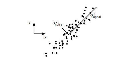
$$SNR=\frac{\sigma _{signal}^{2}}{\sigma _{noise}^{2}}$$

 

A high SNR $(\gg 1)$ indicates a high precision measurement, while a low SNR indicates very noisy data.

2.2.2 Redundancy

Assume the above every 3 plots indicates measurement of an experiment with a different angle.

The left-hand panel depicts two recordings with no apparent relationship which means uncorrelated.

On the other extreme, the right-hand panel depicts highly correlated recordings.

Recoding solely one response would express the data more concisely and reduce the number of sensor recordings.

2.2.3 Covariance Matrix

Consider two sets of measurements with zero means

$A=\left \{ a_{1},a_{2},\cdots ,a_{n} \right \}$, $B=\left \{ b_{1},b_{2},\cdots ,b_{n} \right \}$

 

covariance of $A$ and $B$ $\equiv \sigma _{AB}^{2}=\frac{1}{n}\sum_{i}a_{i}b_{i}$

 

where $\sigma _{AB}=0$ if and only if $A$ and $B$ are uncorrelated

where $\sigma _{AB}^{2}=\sigma _{A}^{2}$ if $A$ = $B$

 

Expressing the covariance as a dot product matrix computation as below.

 

$$\mathbf{a}=\left [ a_{1}a_{2}\cdots a_{n} \right ]$$

$$\mathbf{b}=\left [ b_{1}b_{2}\cdots b_{n} \right ]$$

$$\sigma _{AB}^{2}=\frac{1}{n}\mathbf{ab^{T}}$$

 

Generalize from two vectors to an arbitrary number.

 

$$\mathbf{X=\begin{bmatrix}
x_{1}\\ 
\vdots \\ 
x_{m}
\end{bmatrix}}$$

 

$$\mathbf{C_{X}}=\frac{1}{n}\mathbf{XX^{T}}$$

 

 

where each row of $\mathbf{X}$ corresponds to all measurements of a particular type and $\mathbf{C_{X}}$ is the covariance matrix

 

• $\mathbf{C_{X}}$ is a square symmetric m by m matrix

• The diagonal terms of $\mathbf{C_{X}}$ are the variance of particular measurement types
• The off-diagonal terms of $\mathbf{C_{X}}$ are the covariance between measurement types
• In the diagonal terms, by assumption, large values correspond to an interesting structure
• In the off-diagonal terms, large magnitudes correspond to high redundancy

 

2.2.4 Diagonalize the Covariance Matrix

• All off-diagonal terms in $\mathbf{C_{Y}}$ should be zero. Thus, $\mathbf{C_{Y}}$ must be a diagonal matrix. Or, said another way, $\mathbf{Y}$ is decorrelated
• Each successive dimension in $\mathbf{Y}$ should be rank-ordered according to variance
• Orthonormality assumption gives an efficient, analytical solution to populating ordered a set of $\mathbf{p}$'s which are principal components

 

 

2.3 Solving PCA using eigenvector decomposition

The data set is $\mathbf{X}$, an $m\times n$, where m is the number of measurement types and n is the number of samples.  

 

Find some orthonomal matrix $\mathbf{P}$ in $\mathbf{Y=PX}$ such that $\boldsymbol{C_{Y}}\equiv \frac{1}{n}\boldsymbol{Y}\boldsymbol{Y^{T}}$ is a diagonal matrix. The rows of $\mathbf{P}$ are the principal components of $\mathbf{X}$

 

$$\boldsymbol{C_{Y}}=\frac{1}{n}\boldsymbol{YY^{T}}=\boldsymbol{\frac{1}{n}(PX)(PX)^{T}}=\boldsymbol{P(\frac{1}{n}XX^{T})P^{T}}=\boldsymbol{PC_{X}P^{T}}$$

 

Our plan is to recognize that any symmetric matrix $A$ is diagonalized by an orthogonal matrix of its eigenvectors.

 

For a symmetric matrix $\boldsymbol{A}=\boldsymbol{EDE^{T}}$, where $\boldsymbol{D}$ is a diagonal matrix and $\boldsymbol{E}$ is a matrix of eigenvectors of $\boldsymbol{A}$ arranged as columns. We select the matrix $\boldsymbol{P}$ to be a matrix where each $\boldsymbol{p_{i}}$ is an eigenvector of $\frac{1}{n}\boldsymbol{XX^{Y}}$. By this selection, $\boldsymbol{P}\equiv \boldsymbol{E_{T}}$

$$\boldsymbol{C_{Y}}=\boldsymbol{PC_{X}P^{T}}=\boldsymbol{P(E^{T}DE)P^{T}}=\boldsymbol{P(P^{T}DP)P^{T}}=\boldsymbol{D}$$

 

• For a symmetric matrix A provides A=$EDE^{T}$, where D is a diagonal matrix and E is a matrix of eigenvectors of A arranged as columns 
• The principal components of $\boldsymbol{X}$ are the eigenvectors of $\boldsymbol{C_{X}}=\frac{1}{n}\boldsymbol{XX^{T}}$
• The ith diagonal value of $C_{Y}$ is the variance of $\boldsymbol{X}$ along $\boldsymbol{p_{i}}$

• In practice computing, PCA of a data set $\boldsymbol{X}$ entails
  1. subtracting off the mean of each measurement type
  2. computing the eigenvectors of $\boldsymbol{C_{Y}}$

2.4 Finding optimal $u$

Finding optimal $u$ can formulate as Lagrange multiplier $L(\boldsymbol{u})$

$$L(\boldsymbol{u})=\frac{1}{N}\sum_{i=1}^{N}(\boldsymbol{u^{T}s_{i}-u^{T}\bar{s}})+\lambda (1-\boldsymbol{u^{T}u})$$

 

Differentiate $L(\boldsymbol{u})$ and equate with zero solve optimal $u$

 

$$\frac{\partial L(\boldsymbol{u})}{\partial \boldsymbol{u}}=\frac{\partial \frac{1}{N}\sum_{i=1}^{N}(\boldsymbol{u^{T}s_{i}-u^{T}\bar{s}})+\lambda (1-\boldsymbol{u^{T}u})}{\partial \boldsymbol{u}}=0$$

 

$$=\frac{2}{N}\sum_{i=1}^{N}(\boldsymbol{u^{T}s_{i}-u^{T}\bar{s}})(\boldsymbol{s_{i}-\bar{s}})-2\lambda \boldsymbol{u}=2\boldsymbol{u^{T}}\left ( \frac{1}{N}\sum_{i=1}^{N}(\boldsymbol{s_{i}-\bar{s}})(\boldsymbol{s_{i}-\bar{s}})^{T} \right )-2\lambda \boldsymbol{u}$$

$$=2\boldsymbol{u^{T}\Sigma }-2\lambda \boldsymbol{u}=2\Sigma \boldsymbol{u}-2\lambda \boldsymbol{u}$$

 

$$\Sigma \boldsymbol{u}=\lambda \boldsymbol{u}$$

 

where $\boldsymbol{u}$ is an eigenvector of the covariance matrix $\Sigma$ and $\lambda$ is eigenvalue.

3. Eigendecomposition and Loading Scores

4. Scree plot

Graphical representation of the percentage of variation for each PC account for

4. Application

• Noise filtering
• Visualization
• Feature Extraction
• Stock market predictions
• Gene data analysis
• Quantitative finance
• Neuroscience
• Web indexing
• Meteorology
• Oceanography

5. References

https://arxiv.org/pdf/1404.1100.pdf

https://www.researchgate.net/publication/326541038_A_Tutorial_on_Principal_Component_Analysis_Part_1_Motivation

https://en.wikipedia.org/wiki/Principal_component_analysis

https://onlinecourses.science.psu.edu/stat508/book/export/html/639?source=post_page-----8489b46c2ae0----------------------

https://mccormickml.com/2014/06/03/deep-learning-tutorial-pca-and-whitening/

https://www.youtube.com/watch?v=FgakZw6K1QQ&t=311s

https://medium.com/@jonathan_hui/machine-learning-singular-value-decomposition-svd-principal-component-analysis-pca-1d45e885e491

https://medium.com/@jonathan_hui/machine-learning-linear-algebra-eigenvalue-and-eigenvector-f8d0493564c9