Confidence Interval

1. Overview

2. Description

2.1 Confidence Interval

A confidence interval is a range within which you expect the population parameter to be and its estimation is based on the data we have in our sample. when our confidence is lower the confidence interval itself is smaller. Similarly, for a 99 percent confidence interval, we would have higher confidence but a much larger confidence interval that's an example just to make sure we have solidified this knowledge.

2.1.1 Calculation Confidence Interval

There is a tradeoff between the level of competence we chose and the estimation precision the interval we obtained is broader the opposite is also true. A narrow confidence interval translates to higher uncertainty makes sense right.

2.2 Confidence Level

2.3 Population Unknown

2.4 Margin of Error (ME)

$$Confidence\: Interval=\bar{x}\pm ME$$

Getting a smaller margin of error means that the confidence interval would be narrower as we want a better prediction. It is in our interest to have the narrowest possible confidence interval.

2.4.1 Control the margin of error

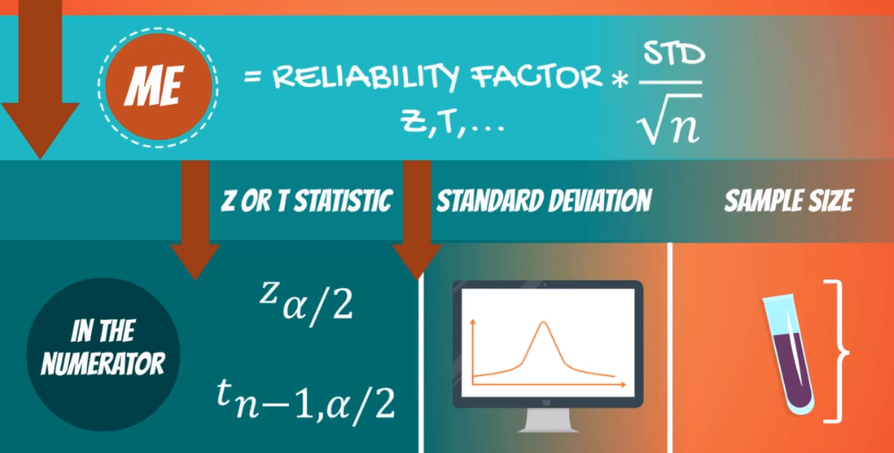
There is a statistic a standard deviation and the sample size statistic and the standard deviation are in the numerator. So smaller statistics and smaller standard deviations will reduce the margin of error. A higher level of confidence increases the statistic. a higher statistic means a higher margin of error. This leads to a wider confidence interval.

A lower standard deviation means that the dataset is more concentrated around the mean. So we have a better chance to get it right.

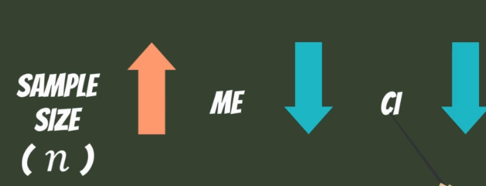
The sample size in the denominator higher sample sizes will decrease the margin of error.

3. Two means, Dependent Samples

The formula that would allow us to calculate a confidence interval is the following. The population is normally distributed but the sample we have contains only 10 observations. Therefore the distribution will have to work with students T and the appropriate statistic is T. You can clearly see that it is the same as the one for a single population with an unknown variance. Let's use the level of confidence and plug in the numbers as we have said many times 95 percent confidence is one of the most common levels.

4. Two means, Independent samples

4.1 Problem 1: Population variance is known

We have a sample of 100 engineering students and the average grade is 58 percent from past years. We know that the population standard deviation is 10 percentage points but the variance is known. We also have a sample of 70 students from the management department and we've got a sample mean of 65 percent again from past data.

• Different departments
• Different teachers
• Different grades
• Different exams

All this information points us to the two samples that are truly independent.

We want to find a 95% confidence interval for the difference between the grades of the students from engineering and management.

• Samples are big
• Population variances are known
• Populations are assumed to follow the normal distribution

All this information points us to the Z statistic instead of the T. 

$$\sigma_{diff}^{2}=\frac{\sigma_{e}^{2}}{n_{e}}+\frac{\sigma_{m}^{2}}{n_{m}}$$

4.2 Problem 2: Population variance unknown but assumed to be equal

Think about this example you were trying to calculate the difference in the price of apples in New York and L.A. you go to ten grocery shops in New York and your friend Paul who lives in L.A. visits grocery shops in order to help you with the research. you don't know what the population variance of apples in New York or L.A. is but you assume it should be the same for NY and L.A. 

We assume that the population variances are equal. So we have to estimate them the unbiased estimate or in this case, is called the pooled sample variance:

$$s_{pooled}^{2}=\frac{(n_{x}-1)s_{x}^{2}+(n_{y}-1)s_{y}^{2}}{n_{x}+n_{y}-2}$$

where the degree of freedom is equal to the total sample size minus the number of variables

• Population variance unknown
• small samples

Using T distribution

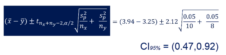
What's the interpretation. We are 95 percent confident that the actual difference between the two populations' price of apples in New York and in L.A. is somewhere between 0.47 and 0.92. Therefore, it is clear that apples in New York are much more expensive than in LA.

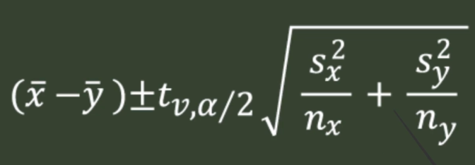
4.3 Problem 3: Population variance unknown but assumed to be different

You can think about comparing apples and oranges. In statistics, if you actually want to compare apples and oranges This is the right way to do it. We have the differences in the means of the two samples the variances or the sample variances of each of the two variables. And here are the respective sample sizes. The tough thing about this is to estimate the degrees of freedom.

4.3.1 Confidence Interval

4.3.2 Degree of freedom

5. Reference

https://365datascience.com/