Ordinary Least Squares Assumptions

1. Overview

If a regression assumption is violated, performing regression analysis will yield an incorrect result. The linear regression is the simplest non-trivial relationship.

2. Linearity

$$\gamma =\beta_{0}+\beta_{1}x_{1}+\beta_{2}x_{2}+\cdots +\beta_{k}x_{k}+\varepsilon $$

How can you verify if the relationship between two variables is linear The easiest way is to choose an independent variable x 1 and plotted against the dependent Y on a scatterplot. If the data points form a pattern that looks like a straight line then a linear regression model is suitable.

If using a linear regression would not be appropriate, fixes for it

• Run a non-linear regression
• Exponential transformation
• Log transformation

The takeaway is if the relationship is nonlinear you should not use the data before transforming it appropriately.

3. No endogeneity

3.1 Omitted variable bias

Omitted variable bias is caused by forgetting to include a relevant variable

Chances are the omitted variable is also correlated with at least one independent X. However you forgot to include it as a regressor. Everything that you don't explain with your model goes into the error. So actually the error becomes correlated with everything else.

3.2 Example

Imagine you're trying to predict the price of an apartment building in London based on its size. This is a rigid model that will have high explanatory power. However, from our sample it seems that the smaller the size of the houses the higher the price. This is extremely counterintuitive. it seems that the covariance of the independent variables and the error terms is not 0.

We omitted the exact location as a variable in almost any other city. This would not be a factor but in our particular example the million-dollar suites in the city of London turn things around after we included a variable that measures if the property is in London city.

The easiest way to detect an omitted variable bias is through the error term. Only experience and advanced knowledge can help.

4. Normality and homoscedasticity

$$\varepsilon \sim N(0,\sigma ^{2})$$

4.1 Normality

We assume the error term is normally distributed normal distribution is not required for creating the regression but for making inferences. all regression tables were full of statistics and F's sticks. These things work because we assume normality of the error term What should we do if the error. The central limit theorem applies for the error terms too. Therefore we can consider normality as a given for us.

4.2 Zero mean

A zero mean of error terms. If the mean is not expected to be 0 then the line is not the best fitting one. However, having an intercept solves that problem.

4.3 Homoscedasticity

$H_{0}$ have equal variance

$$\sigma_{\varepsilon_{1}}^{2}=\sigma_{\varepsilon_{2}}^{2}=\cdots =\sigma_{\varepsilon_{k}}^{2}=\sigma^{2}$$

What if there was a pattern in the variance. An example of a data set where errors have a different variance. It looks like this starting close to the regression line and going further away.

4.3.1 Prevention

• Look for omitted variable bias
• Look for outliers
• Log transformation: Create a regression between the log of Y and the independent X's. Conversely, you can take the independent X that is causing you trouble and do the same.

4.3.2 Example

This is a scatterplot that represents a high level of heteroscedasticity. On the left-hand side of the chart, The variance of the error is small while on the right it is high.

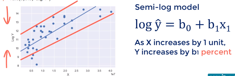
let's transform the experiential to a new variable called log of X and plot the data. This is the new result. Changing the scale of x would reduce the width of the graph. You can see how the points came closer to each other from left to right. The new model is called a semi-log model.

What if we transform the Y scale instead and n logically to what happened previously. We would expect the height of the graph to be reduced and that's the result. This looks like good linear regression material doesn't it. The hetero's get asked in-city we observed earlier is almost gone. This new model is also called the semi-log model its meaning is as x increases by one unit Y changes by B 1%.

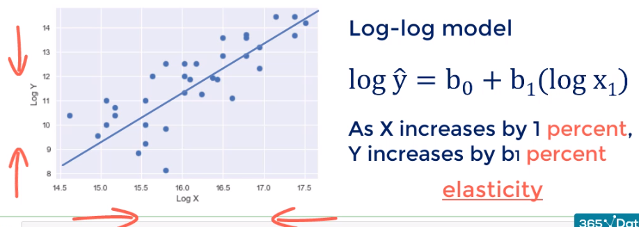
Sometimes we want or need to change both scales to log. The result is a log-log model. We shrink the graph in height and in with this is the result the improvement is noticeable but not game-changing. The interpretation is for each percentage point change and X Y changes by b1 percentage points. If you've done economics you would recognize such a relationship is known as elasticity.

5. No autocorrelation (Independence of errors)

It is also known as no serial correlation. Autocorrelation is not observed in cross-sectional data.

$$\sigma_{\varepsilon_{i}\varepsilon_{j}}=0:\forall i\neq j$$

Errors are assumed to be uncorrelated. Where can we observe a serial correlation between errors? It is highly unlikely to find it in data taken at one moment of time known as cross-sectional data. However, it is very common in time-series data.

5.1 Example

Think about stock prices. Every day you have a new quote for the same stock. These new numbers you see have the same underlying asset. Ideally, you want them to be random or predicted by macro factors such as GDP tax rate political events and so on. Unfortunately, it is common in underdeveloped markets to see patterns in the stock prices.

5.2 Detection

Durbin-Watson falls are between 0 and 4. If 2, no autocorrelation. If smaller than 1 and larger than 3, It causes an alarm.

5.3 No Remedy

When in the presence of autocorrelation avoid the linear regression model.

5.3.1 Alternatives

• Autoregressive model
• Moving average model
• The autoregressive moving average model
• The autoregressive integrated moving average model

6. No multicollinearity

We observe multicollinearity when two or more variables have a high correlation.

$$\rho_{x_{i}x_{j}}\approx 1:\forall i,j;i\neq j$$

This imposes a big problem to our regression model as the coefficients will be wrongly estimated. The reasoning is that if a can be represented using B there is no point using both. We can just keep one of them.

Another example would be two variables C and D with a correlation of 90 percent. If we had a regression model using C and D We would also have multi-collinearity although not perfect here.  The assumption is still violated and poses a problem to our model.

6.1 Example

A regression-based on these three variables the p-value for the pint of beer at bonkers and half a bound bonkers show they are insignificant. why? the underlying logic behind our model was The price of half a pint and a full pint that bonkers definitely moved together this messed up the calculations of the computer and it provided us with wrong estimates and wrong p-values.

6.2 Fixes

• Drop one of the two variables.
• Transform them into one variable.
• If you are super confident in your skills you can keep them both while treating them with extreme caution.

6.3 Prevention

Find the correlation between every two pairs of independent variables

$$\rho_{x_{i}x_{j}}\approx 1:\forall i,j;i\neq j$$

7. Reference

https://www.statisticssolutions.com/homoscedasticity/