Least-squares for model fitting

1. Overview

There are uncountable dynamics and processes and individuals with uncountable and mind-bogglingly complex interactions. So how can we possibly make sense of all of this complexity? The answer is we can't :(

So instead we generate simple models and we fit models to data using linear least squares modeling and that is the goal of this section of the course.

the idea of building models is that instead of trying to understand the un-understandable complexity of the universe we build simplified models of the most important aspects of the system under investigation. Now, this eventually leads to a model and a model is a set of equations that allows us, scientists, to isolate and understand important principles of the system while ignoring other parts of the system that might be less relevant.

 

2. Description

2.1 Model fitting Intuition

The goal is not to replicate exactly the system under investigation but instead to identify a simplified and low dimensional representation that actually can be understood and worked with. Now, on the other hand, there is a lot of diversity in nature and models should be sufficiently generic that they can be applied to many different datasets. So we need a way to make the models flexible enough that they can be adjusted to different datasets without having to create a brand new model for each particular dataset.

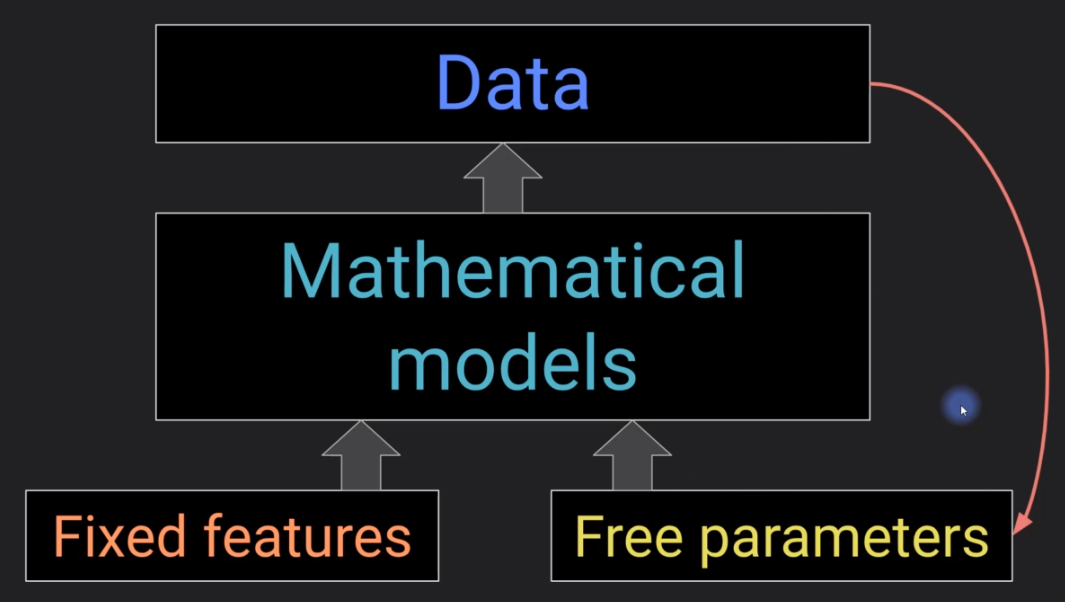
Fixed Features: The fixed features are components of the model that you impose on the model based on your knowledge based on scientific evidence, based on theories.

Free parameters: Now free parameters, on the other hand, are variables that can be adjusted to fit any particular data set or any specific set of data points. And this is the primary goal of model fitting -- first to come up with a model and then to adjust the values of these free parameters so that they match the data. This is called model fitting. The most commonly used method for model fitting is called linear least squares.

2.2 Model fitting procedure

2.2.1 Define the equation(s) underlying the model

Let's say you want to predict how tall someone is. So you might come up with an equation that looks like this. This is the outcome measure sometimes called the dependent variable. And this is height and then you say that height is the result of the sex.

Now obviously what really determines someone's height is way way more complicated than this model but this model captures a few of the important factors in a simplistic way and that is the goal here.

These betas here beta one beta two beta 3. These are the free parameters. These are the parameters that we are going to fit the data and these terms here. Sex parents' height and childhood nutrition. These are the fixed features in the model.

2.2.2 Map the data into the model equations

Notice that each of these equations follows the same template just that the numbers are different for each individual. And here this is 1 or 0. This is called dummy coding that's typically done in statistics to deal with binary variables like this.

Now actually there is one component that's missing from this model and that is the intercept which captures the expected value of the data when all of these predictors are zero.

2.2.3 Convert the equations into a matrix-vector equation

2.2.4 Compute the parameters

2.2.5 Statistical evaluation of the model

3. The terminology of linear algebra

4. Reference