-
Artificial neural network(ANN)MLAI/DeepLearning 2019. 10. 5. 13:39
1. Overview
Artificial neural networks (ANN) or connectionist systems are computing systems that are inspired by, but not identical to, biological neural networks that constitute animal brains. Such systems "learn" to perform tasks by considering examples, generally without being programmed with task-specific rules. For example, in image recognition, they might learn to identify images that contain cats by analyzing example images that have been manually labeled as "cat" or "no cat" and using the results to identify cats in other images. They do this without any prior knowledge of cats, for example, that they have fur, tails, whiskers and cat-like faces. Instead, they automatically generate identifying characteristics from the examples that they process.
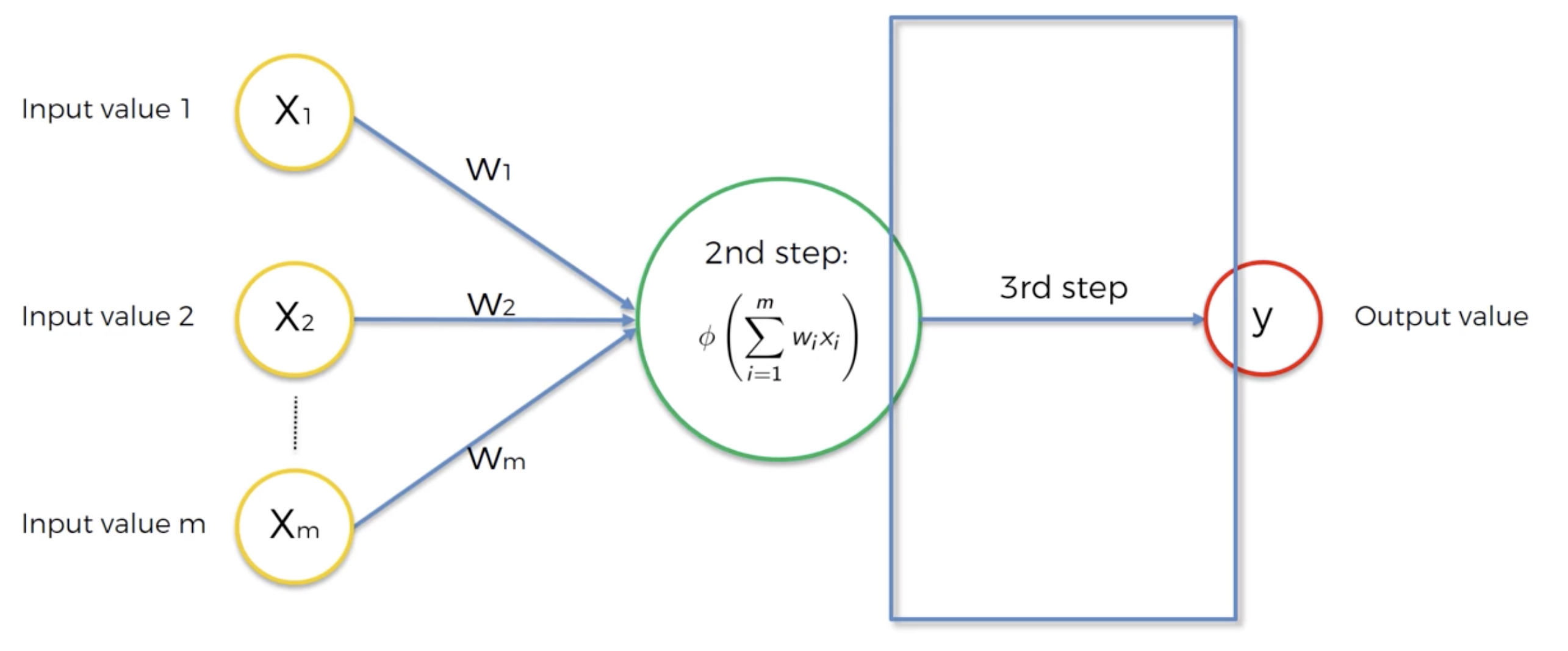
An ANN is based on a collection of connected units or nodes called artificial neurons, which loosely model the neurons in a biological brain. Each connection, like the synapses in a biological brain, can transmit a signal to other neurons. An artificial neuron that receives a signal then processes it and can signal neurons connected to it.
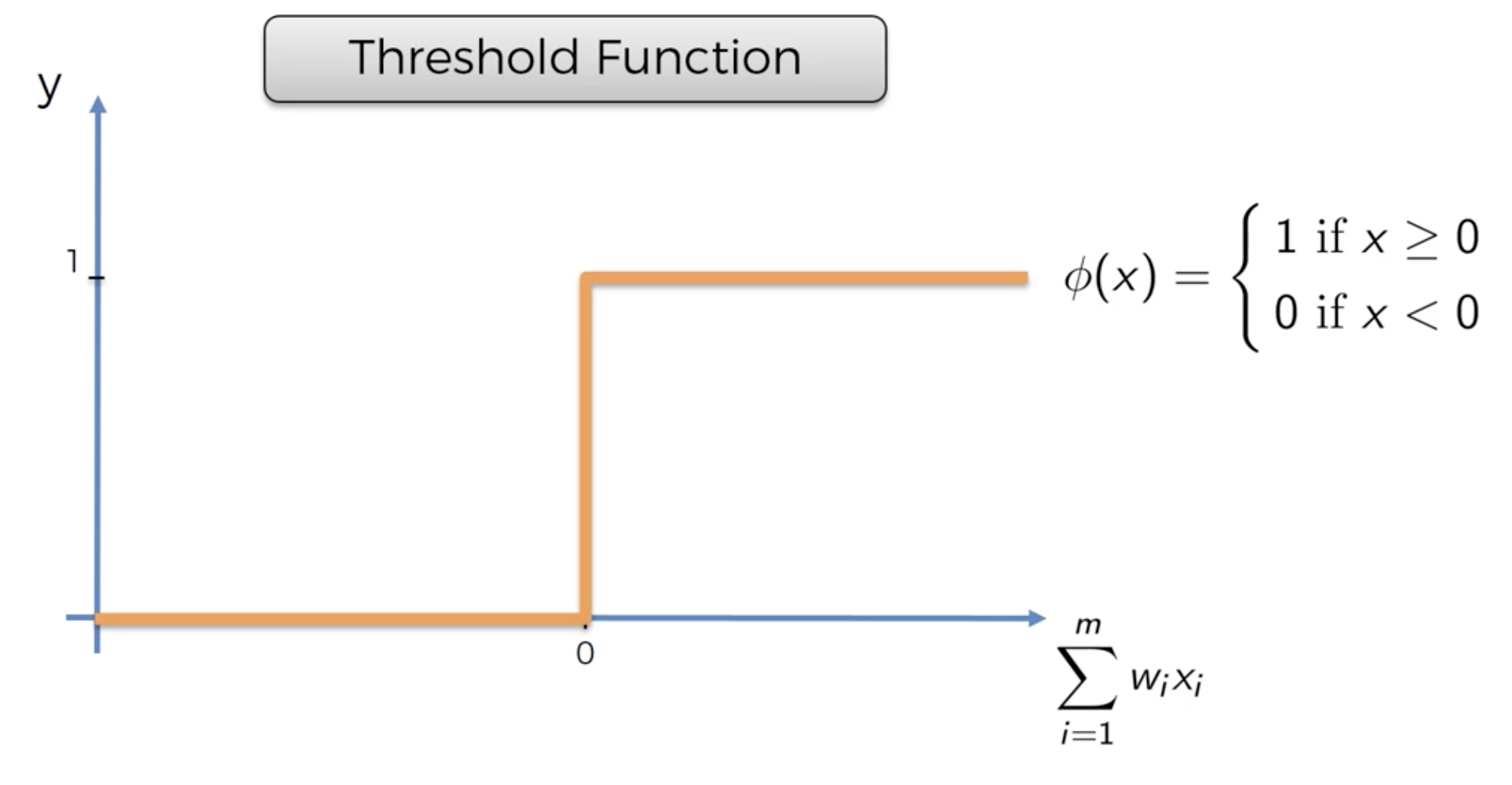
In ANN implementations, the "signal" at a connection is a real number, and the output of each neuron is computed by some non-linear function of the sum of its inputs. The connections are called edges. Neurons and edges typically have a weight that adjusts as learning proceeds. The weight increases or decreases the strength of the signal at a connection. Neurons may have a threshold such that a signal is sent only if the aggregate signal crosses that threshold. Typically, neurons are aggregated into layers. Different layers may perform different transformations on their inputs. Signals travel from the first layer (the input layer), to the last layer (the output layer), possibly after traversing the layers multiple times.
The original goal of the ANN approach was to solve problems in the same way that a human brain would. However, over time, attention moved to performing specific tasks, leading to deviations from biology. ANNs have been used on a variety of tasks, including computer vision, speech recognition, machine translation, social network filtering, playing board and video games, medical diagnosis and even in activities that have traditionally been considered as reserved to humans, like painting
2. Description
2.1 Neuron

2.2 Activation function
2.2.1 Threshold function
2.2.2 Sigmoid function

Similar with logistic regression
2.2.3 Rectifier function

2.2.4 Hyperbolic tangent function(tanh)
2.3 Work procedure
2.3.1 Without hidden layer

2.3.2 With hidden layer

Hidden layers allows you to increase the flexibility of neural network to look for very specific things and then in combination, that's where the power comes from.
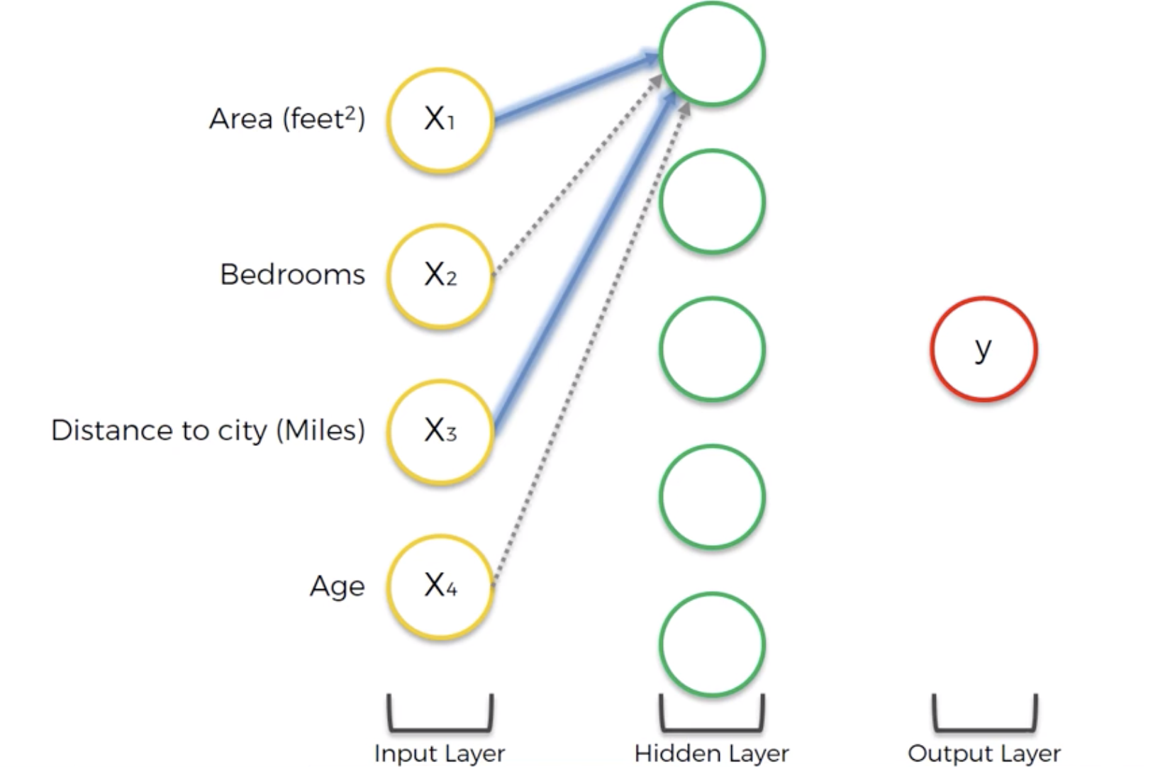
A neuron associated with Area and Distance to city, but not bedrooms and age for output price.

A neuron associated with Area, Bedroom, and Age which is probably trained by the set there's a lot of families want many bedrooms and new(young) house.

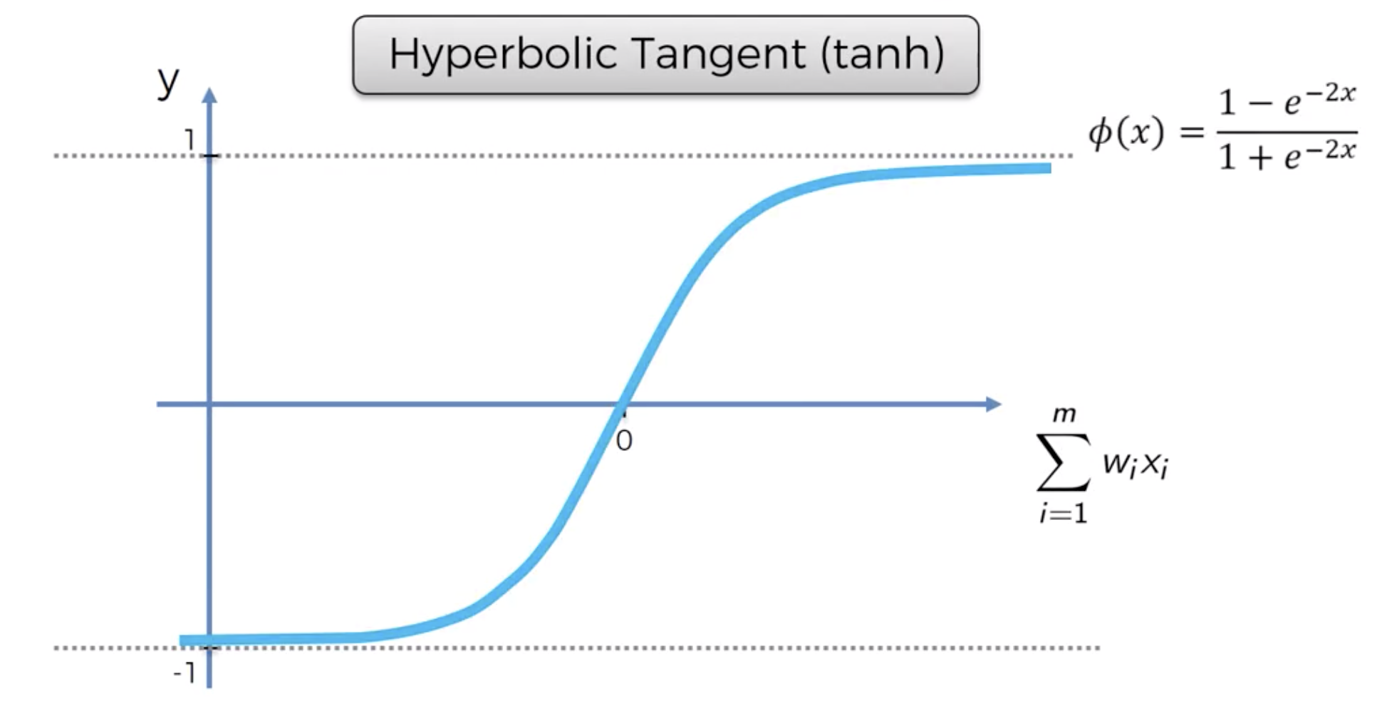
As usually, Old building is less valuable because it's worn out, things are falling apart, and more maintenance is requried. So price drops in terms of the price of real estate as age goes on. But if age jumps over 100 years old, it become historical property which means valuable. In this case, the rectifier function being applied.

Combination of Bedrooms and Distance to city contribute price, but it's not as strong as the other neurons.
3. Learning
3.1 Single Data

3.1 Cost function
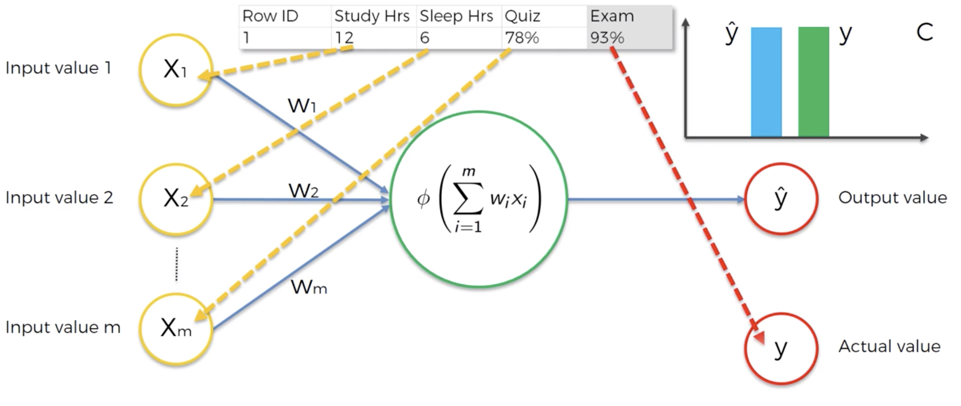
What is the error that you have in your prediction and our goal is to minimize the cost function because the lower cost function the closer the $\hat{y}$ is to y.

Once comparing the $\hat{y}$ and y, now going to feed this information back into the neural network and goes to weights and the weights get updated. In this scenario, The only thing to control is weights.
3.2 Multi-data and one Neural network

3.2.1 Back propagation
Iterate calcurating cost function and updating weights per each epoch till cost function lowering enough that satisfy some condition.
3.3 Training the ANN with stochastic gradient descent
Step 1: Randomly initialise the weights to small numbers close to 0, but not 0
Step 2: Input the first observation of your dataset in the input layer. each feature in one input node.
Step 3: Forward-Propagation: from left to right, the neurons are activated in a way that the impact of each neuron's activation is limited by the weights. Propage the activations until getting the predicted result $\hat{y}$
Step 4: Compare the predicted result to the actual result y. Measure the generated error.Step 5: Back-propagation: from right to left, the error is back-propagated. Update the weights according to how much they are responsible for the error. The learning rate decides by how much we update the weights.
Step 6: Repeat Steps 1 to 5 and update the weights after each observation (Reinforment Learning). Or: Repeat Steps 1 to 5 but update the weights only after a batch of observations (Batch Learning).
Step 7: When the whole training set passed through the ANN, that makes an epoch. Redo more epochs.
4. Gradient descent

4.1 Curse of dimensionality

4.1.1 brute force way
Assuming 1000 combinations:

4.1.2 (batch) Gradient of convex cost function


4.2 Stochastic gradient descent(SGD)


Help of stocahstic gradient descent is avoiding local solution of gradient descent cause of higher fluctuation which is much more likely to find the global minimun rather than just local minimum.
Also it's faster than batch gradient descent because it doesn't load up all the data into memory and run and wait until all those row are run altogether, so much lighter algorithm.
The main advantage is that it is a deterministic algorithm meaning it's random. With the batch gradient descent method, as long as you have the same starting weights for your neural networks, every time you run the batch gradient descent method, you will get the same iterations and the same results for the way your weights are being updated. For the stochastic gradient descent method, you won't get that because picking your rows possible at random and you are updating your neural network in a stochastic manner and therefore even same weights start points, you're going to have different process.
4.2.1 Mini-batch gradient descent method
Middle of batch and stochastic method.
4.3 Forward and Backward propagation

4.3.1 Forward propagation
Where information is entered into the input layer, and then is propagated forward to get $\hat{y}$. And compare it with actual y to calculate the errors.
4.3.2 Backward propagation

The errors are back-propagated through the network in the opposite direction that allows to train the network by adjusting the weights. Backpropagation is an advanced algorithm driven by sophisticated mathematics which allows us to adjust the weights, all of them at the same time.
During the process of backpropagation, Simply because of the way the algorithm is structured, you are able to adjust all of the weights at the same time. So you basically know which part of the error each of your weights in the neural network is responsible for.
5. Example
5.1 Activation function
5.1.1 Binary input

5.1.2 Multi-layered activation function

6. References
http://static.latexstudio.net/article/2018/0912/neuralnetworksanddeeplearning.pdf
https://iamtrask.github.io/2015/07/12/basic-python-network/
https://iamtrask.github.io/2015/07/27/python-network-part2/
https://en.wikipedia.org/wiki/Perceptron
https://en.wikipedia.org/wiki/Artificial_neural_network
https://www.superdatascience.com/
http://yann.lecun.com/exdb/publis/pdf/lecun-98b.pdf
'MLAI > DeepLearning' 카테고리의 다른 글
Boltzmann Machine with Energy-Based Models and Restricted Boltzmann machines(RBM) (0) 2019.10.19 Classify Deep Learning (0) 2019.10.16 Softmax and Cross-Entropy with CNN (0) 2019.10.16 Convolutional Neural Networks(CNN) (0) 2019.09.30 Difference between Deep Learning and Shallow learning (0) 2019.09.25