Hidden Markov Model(HMM)

1. Overview

HMM is called hidden because only the symbols emitted by the system are observable, not the underlying random walk between states. An HMM can be visualized as a finite state machine. it generates a protein sequence by emitting amino acids as it progresses through a series of states. 

2. Description

2.1 Definition of Markov Model

 

There are four common Markov models used in different situations, depending on whether every sequential state is observable or not, and whether the system is to be adjusted on the basis of observations made:

	The system state is fully observable	The system state is partially observable
System is autonomous	Markov chain	Hidden Markov model
System is controlled	Markov decision process	Partially observable Markov decision process

2.1.1 Markov Chain

A Markov chain is a stochastic model describing a sequence of possible events in which the probability of each event depends only on the state attained in the previous event.

A Markov chain with memory(or a Markov chain of order m)

$$P(X_{n}=x_{n}\, |\, X_{n-1}=x_{n-1},X_{n-1}=x_{n-1},\cdots ,X_{n-m}=x_{n-m})\,  for\,  n > m$$

 

2.1.2 Markov assumption

$$P(o_{i}\, |\, o_{i-1},\cdots ,o_{1})=P(o_{i}\, |\, o_{i-1})$$

2.2 Definition of Hidden Markov Model(HMM)

Hidden Markov Model (HMM) is a statistical Markov model in which the system being modeled is assumed to be a Markov process with unobservable (i.e. hidden) states. The states of an HMM are hidden and can only be inferred from the observed symbols.

Let $X_{n}$ and $Y_{n}$ be discrete-time stochastic processes and $n \geq 1$. The pair $\left ( X_{n}, Y_{n} \right )$ is a Hidden Markov model if

• $X_{n}$ is a Markov process and is not directly observable which means hidden
• $\mathbf{P}(Y_{n}\in A\, |\, X_{1}=x_{1},\cdots ,X_{n}=x_{n})=\mathbf{P}(Y_{n}\in A\, |\, X_{n} = x_{n})$

for every $n \geq 1,\,  x_{1},\cdots ,x_{n}$, and an arbitrary measurable set A

The states of the process $X_{n}$ are called hidden states

$\mathbf{P}(Y_{n}\in A\, |\, X_{n} = x_{n})$ is called an emission probability or output probability

2.3 Notation of HMM

Three sets of parameters $\lambda = (\pi , A, B)$

2.3.1 Initial state probabilities $\pi$

$$\pi _{i} = P(q_{1}=S_{i})$$

where $\pi _{i}\, \geq 0,\,  \sum_{i=1}^{N}\pi _{i}=1$

2.3.2 Transition probabilities $\mathit{A}$

$$A= a_{ij} = P(X_{t+1} = j\, |\, X_{t}=i)$$

where $a _{ij}\, \geq 0,\,  \sum_{j=1}^{N}a _{ij}=1$

2.3.2 Transition probabilities $\mathit{B}$

$$B=b_{j}(v)=P(o_{t}=v\, |\, X_{t}=j)$$

where $b _{j}(v)\, \geq 0,\,  \sum_{v\,  \in \, V}b_{j}(v)=1$

2.4 Three Problems

2.4.1 Evaluation

Q: Given the observation sequence $O=O_{1}O_{2}\cdots O_{T}$, and a model $\lambda =(A,B,\pi )$, how do we efficiently compute $P(O|\lambda )$, the probability of the observation sequence, given the model

A: Forward Algorithm, Backward Algorithm

 

• Forward Algorithm

The forward algorithm, in the context of a hidden Markov model (HMM), is used to calculate a 'belief state': the probability of a state at a certain time, given the history of evidence. The process is also known as filtering. The forward algorithm is closely related to, but distinct from, the Viterbi algorithm.

• Definition

$$\alpha (i)=P(o_{1}\cdots o_{t},q_{t} =s_{i}\, |\, \lambda )$$

 

• Process

Initialization

$$\alpha (i)=\pi _{i}b_{i}(o_{1})$$

 

Inductive definition

$$\alpha (j)=\left [ \sum_{i=1}^{N} \alpha _{t-1}(i)a_{ij} \right ]b_{j}(o_{t})$$

where $(2\leq t\leq T, 1\leq j\leq N)$

2.4.2 Encoding

Q: Given the observation sequence $O=O_{1}O_{2}\cdots O_{T}$, and a model $\lambda =(A,B,\pi )$, how do we choose a corresponding state sequence $Q=q_{1}q_{2}\cdots q_{T}$ which is optimal in some meaningful sense(i.e., best explains the observations)

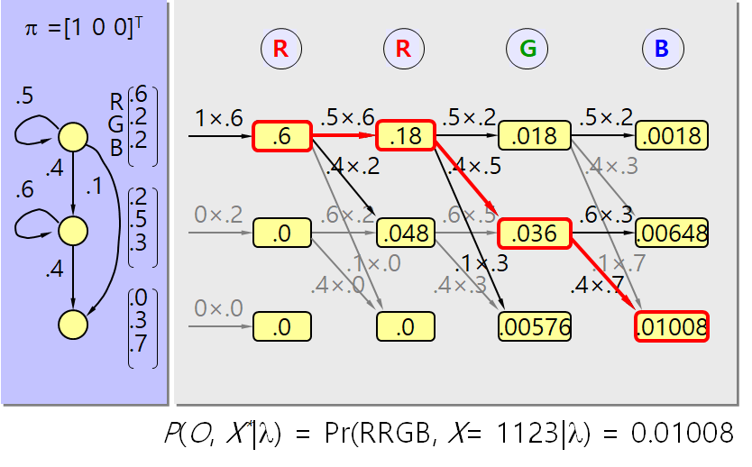
A: Viterbi Algorithm

 

Is the path whose joint probability with the observation is the most likely:

$$\hat{X}_{1,T}=\underset{X}{argmax}P(O,X\, |\, \lambda )$$

 

Simplistic rewriting:

$$P(O,X\, |\, \lambda )=P(O\, |\, X,\lambda )P(X\, |\, \lambda )$$

$$=\pi _{x_{1}}a _{x_{1}x_{2}}a _{x_{2}x_{3}}\cdots a _{x_{T-1}x_{T}}\times b_{x_{1}}(o_{1})b_{x_{2}}(o_{2})\cdots b_{x_{T}}(o_{T})$$

 

where $O(TN^{T})$ multiplications with exhaustive enumeration

 

• Viterbi Algorithm

The Viterbi algorithm is a dynamic programming algorithm for finding the most likely sequence of hidden states—called the Viterbi path—that results in a sequence of observed events, especially in the context of Markov information sources and hidden Markov models(HMM)

 

• Initialization

$$\delta _{1}(i)=\pi _{i}b_{i}(o_{1})$$

$$\psi  _{1}(i)=0$$

• Recursion

$$\delta _{t+1}(j)=\underset{1\leq i\leq N}{max}\delta _{t}(i)a_{ij}b_{j}(o_{t+1})$$

$$\psi  _{t+1}(j)=\underset{1\leq i\leq N}{argmax}\, \delta _{t}(i)\, a_{ij}$$

• Termination

$$P^{*}=\underset{1\leq i\leq N}{max}\delta _{T}(i)$$

$$x_{T}^{*}=\underset{1\leq i\leq N}{argmax}\, \delta _{T}(i)$$

• Backtracing

$$x_{t}^{*}=\psi _{t+1}(x_{t+1}^{*})$$

where $t=T-1, \cdots , 1$

• Example

2.4.3 Learning

Q: How do we adjust the model parameters $\lambda =(A,B,\pi )$ to maximize $P(O|\lambda )$

A: Baum-Welch Algorithm

 

• Definition of $\xi _{t}(i,j)$

The probability of being in a state $S_i$ at time t, and state $S_j$ at time t + 1, given the model and the observation sequence

 

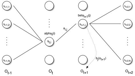
$$\xi _{t}(i,j)=P(q_{t}=s_{i},q_{t+1}=s_{j}\, |\, O,\lambda )=\frac{\alpha _{t}(i)a_{i,j}b_{j}(o_{t+1})\beta _{t+1}(j)}{\sum_{i=1}^{N}\sum_{j=1}^{N}\alpha _{t}(i)a_{i,j}b_{j}(o_{t+1})\beta _{t+1}(j)}$$

 

• Definition of $\gamma _{t}(i)$

The probability of being in state $S_{i}$ at time t, given the observation sequence and the model

$$\gamma _{t}(i)=P(q_{t}=s_{i}\, |\, O,\lambda )=\sum_{j=1}^{N}\xi _{t}(i,j)$$

 

• Reestimation

$\bar{\pi }$ = expected frequency (number of times) from state $S_{i}$ to state $S_{j}$

 

$$\bar{a_{ij}}=\frac{\sum_{t=1}^{T-1}\xi _{t}(i,j)}{\sum_{t=1}^{T-1}\gamma _{t}(i)}$$

where $\sum_{t=1}^{T-1}\xi _{t}(i,j)$ is expected number of transitions from state $S_{i}$ to state $S_{j}$ and $\sum_{t=1}^{T-1}\gamma _{t}(i)$ is expected number of transitions from state $S_{i}$

 

$$\bar{b_{i}}(k)=\frac{\underset{s.t. O_{t}=v_{k}}{\sum_{t=1}^{T}}\gamma _{t}(j)}{\sum_{t=1}^{T-1}\gamma _{t}(j)}$$

where $\underset{s.t. O_{t}=v_{k}}{\sum_{t=1}^{T}}\gamma _{t}(j)$ expected number of times in state j and observing symbol $v_{k}$ and $\sum_{t=1}^{T-1}\gamma _{t}(j)$ expected number of times in state j

 

$\bar{\lambda }=(\bar{A},\bar{B},\bar{\pi })$

 

The reestimation formulas can be derived directly by maximizing Baum's auxiliary function

$$Q(\lambda ,\bar{\lambda })=\sum_{Q}P(Q\, |\, O,\lambda )log\left [ P(O,Q\, |\, \bar{\lambda }) \right ]$$

 

over $\bar{\lambda }$. It has been proven by Baum that maximization of $Q(\lambda, \bar{\lambda })$ leads to increased likelihood, i.e.

 

$$\underset{\bar{\lambda }}{max}\left [ Q(\lambda ,\bar{\lambda }) \right ]\Rightarrow P(O\, |\, \bar{\lambda })\geq P(O\, |\, \lambda )$$

3. Evaluation

3.1 Advantages

• Strong statistical foundation
• Efficient learning algorithms.
  • Learning can take place directly from raw sequence data
• Allow consistently treatment of insertion and deletion penalties in the form of locally learnable
• Can handle inputs of variable length
  • They are the most flexible generalization of sequence profiles
• Wide variety of applications including multiple alignments, data mining and classification, structural analysis, and pattern discovery
• Can be combined into libraries

3.2 Disadvantages

• First-order HMMs are limited by their first-order Markov property
• They cannot express dependencies between hidden states
• HMMs often have a large number of unstructured parameters
• Proteins fold into complex 3-D shapes determining their function
• The HMM is unable to capture higher-order correlation among amino acids in a protein molecule
• Only a small fraction of distributions over the space of possible sequences can be represented by a reasonably constrained HMM

3.3 Application

• Identification of G-protein coupled receptors
• Clustering of paths for a subgroup
• Gene prediction
• Modeling protein domains

4. References

https://www.ece.ucsb.edu/Faculty/Rabiner/ece259/Reprints/tutorial%20on%20hmm%20and%20applications.pdf

https://pomegranate.readthedocs.io/en/latest/HiddenMarkovModel.html

https://www.slideshare.net/joshiblog/advantages-and-disadvantages-of-hidden-markov-model

https://www.researchgate.net/post/When_is_it_better_to_use_Hidden_Markov_Model_instead_of_other_pattern_recognition_techniques

https://link.springer.com/chapter/10.1007/978-1-4302-5990-9_5

https://en.wikipedia.org/wiki/Hidden_Markov_model

https://en.wikipedia.org/wiki/Markov_chain#targetText=A%20Markov%20chain%20is%20a,attained%20in%20the%20previous%20event.&targetText=Markov%20studied%20Markov%20processes%20in,on%20the%20topic%20in%201906.

https://en.wikipedia.org/wiki/Markov_property#targetText=The%20term%20Markov%20assumption%20is,an%20interconnected%20network%20of%20items.

https://en.wikipedia.org/wiki/Viterbi_algorithm#targetText=The%20Viterbi%20algorithm%20is%20a,hidden%20Markov%20models%20(HMM).

https://en.wikipedia.org/wiki/Forward_algorithm

https://www.quora.com/What-is-the-difference-between-Markov-Models-and-Hidden-Markov-Models

https://www.youtube.com/watch?v=K-ck5dOsPgQ

https://stackoverflow.com/questions/10748426/what-is-the-difference-between-markov-chains-and-hidden-markov-model