Naive Bayes classifier

1. Overview

2. Bayes Theorem

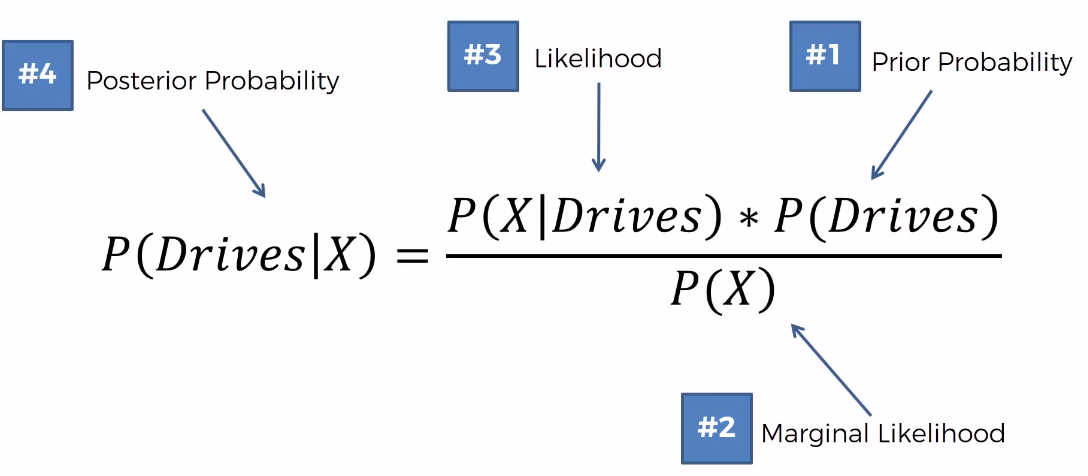
2.1 Formula

$$P(A|B)=\frac{P(B|A)\times P(A)}{P(B)}$$

2.2 Example

3. Classifier

3.1 Procedure

3.1.1 Step 1

3.1.2 Step 2

3.1.3 Step 3

 

The first time we're going to apply it to find out what is the probability that this person walks given his features and X over here is the features or presents the features of that data point.

And then we're going to look at all the points that are inside this series and what we're saying here is that all of the points inside the circle are we going to deem them to be similar in terms of features to the point that we had.

Remember it had an age of for example 25 and a salary of $30000 per year. So now we're going to draw a radius around it and let's say anybody between the age of 20 and 30 and in the salaries of $25000 to $35000.

Anybody that falls in that circle again is it's not a square it's a square is a circle. Anybody who falls somewhere is somewhere in that vicinity is going to be deemed similar to the new data point that we're adding to our data set.

2.1 Prior Probability

The number of people that actually walk and divide by the overall number so probably that person walks to work with the number of walkers and number of people or walk which is these are dots divided by the total number absorption the green dots are the gray dot isn't participating in these calculations.

So here we have probably if somebody walks are 10 red dots divide by 30 dots overall.

2.2 Marginal Likelihood

The probability that any random point to fall into this circle and P of X is calculated as the number of similar observations so the number of observations that already we can see in the circle.

2.3 Likelihood

the question is given that we're only working with the red dots What is the likelihood that a randomly selected data point from our dataset from the red dots is somebody who exhibits features similar to the point that we are adding to our dataset. So basically what is the likelihood that a randomly selected red dot falls into this gray area into the circle.

75% is the probability that somebody that we put into the place where we're putting X is should be classified as a person who walks to work.

The probability of somebody who exhibits features X being a person who drives to work is 25%.

4. Intuition

4.1 Naive Bayesian

Why is this algorithm called the native base algorithm? The answer is because the Bayes theorem requires some independent assumptions and the base theorem is the foundation of the Navy base machine learning algorithm and therefore the naive Bayes machine learning algorithm also relies on these assumptions which are oftentimes not correct and therefore it's kind of naive to assume that they're going to be correct. Independent assumption. That's why it's called naive because it's a naive assumption.

Bayes theorem the way we apply it actually requires that age and salary have to be independent of the variables that we're working with. In this case, is your salary has to be independent and that is like a fundamental assumption of the base theorem and then you can only apply it and then you can't get those probabilities and so on.

And therefore given that they are not independent you can't really apply the Bayes Theorem and therefore you can apply the base algorithm to machine learning and that's why it's called Neive a base algorithm because oftentimes it's applied even though the variables or the features are not independent or not completely independent and it's still applied and it still gives good results.

4.2 P(X)

P(X) is the likelihood that a randomly selected point from this dataset will exhibit features similar to the data point that we are about to add. And as we agreed on anything in that circle is deemed to be similar to our data point.

And that way we won't actually have to perform that calculation. So that's one less calculation to perform. So you can just compare the top part of these calculations and so that is what is done a lot of the time. It's totally valid to do it that way but that is only if you're comparing the two. Right if you're only comparing the two then you can do that if you actually wanted to calculate the value.

4.3 More than 2 classes

it's very straightforward. And moreover, you'll find that every time when you just have two classes it'll always add up to one. So we didn't even have to calculate the second one.

5. References

https://en.wikipedia.org/wiki/Naive_Bayes_classifier