Simple Linear Regression

1. Overview

Linear regression attempts to model the relationship between two variables by fitting a linear equation to observed data. One variable is considered to be an explanatory variable, and the other is considered to be a dependent variable. For example, a modeler might want to relate the weights of individuals to their heights using a linear regression model.

2. Description

2.1 Process

• Get sample data
• Design a model that works for that sample
• Make predictions for the whole population

2.1 Formula

2.1.1 Population formula

2.1.2 Sample formula

The unit changes a unit change in $x_{1}$ how that affects a unit change in y. So it's kind of think of it as the translator or the multiplier or something like that that that's connects to the connector between y and $x_{1}$ so you can always say $x_{1}$ is directly proportional

2.2 Learning: Ordinary least squares (OLS)

To get this best-fitting line what is done is you take the sum you take each one of those green lines are those distances you square them and then you take some of those squares. Once you have the sum of the squares for you got to find the minimum.

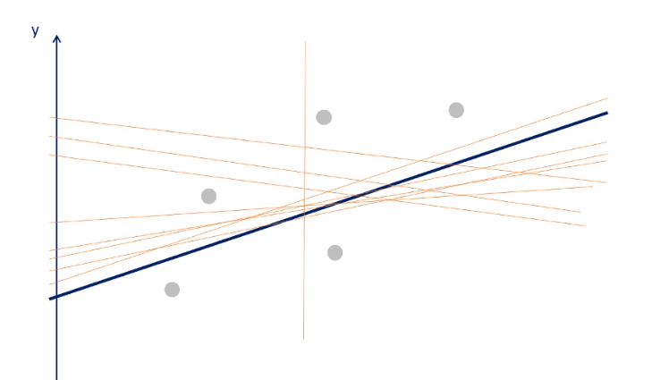
So basically what a simple linear regression does is it draws lots and lots and lots of these lines. The linear regression draws all these all possible trend trendlines and counts the sum of those squares every single time and then it finds the minimum one so it looks for the minimum sum of squares and finds a line that has the smallest sum of squares possible. And that line will be the best fitting line and that is called the ordinary least squares method.

A lower error results in a better explanatory power of the regression model. So this method aims to find the line which minimizes the sum of the squared errors.

2.2.1 OLSM Formulation

$$\hat{b}=\underset{b}{argmin}\: S(b)$$

where $S(b)=\sum_{i=1}^{n}(y_{i}-x_{i}^{T}b)^{2}=(y-Xb)^{T}(y-Xb)$

this is a minimization problem that uses calculus and linear algebra to determine the slope and intercept of the line.

3. Determinants

3.1 Sum of Squares Total (SST, Toal sum of squares, TSS)

$$\sum_{i=1}^{n}(y_{i}-\bar{y})^{2}$$

It is the square of the difference between the observed dependent variable and its mean. The dispersion of the observed variables around the mean. It is a measure of the total variability of the data set.

3.2 Sum of squares regression (SSR, Explain Sum of squares, ESS)

$$\sum_{i=1}^{n}(\hat{y}_{i}-\bar{y})^{2}$$

It is the sum of the differences between the predicted value and the mean of the dependent variable. Think of it as a measure that describes how well your line fits the data. If this value of SSR is equal to the sum of squares total, which is SSR = SST, It means your regression model captures all the observed variability and is perfect.

3.3 Sum of squares error (SSE, Residual Sum of squares, RSS)

$$\sum_{i=1}^{n}e_{i}^{2}$$

The error is the difference between the observed value and the predicted value. The smaller the error the better the estimation power of the regression. Measures the unexplained variability by the regression.

3.4 Coefficient of Determination $R^{2}$

$$\frac{SSR}{SST}$$

It is a relative measure and takes values ranging from 0 to 1. and R squared of 0 means your regression line explains none of the variability of the data. And, R-squared of 1 would mean your model explains the entire variability of the data. 

The R squared measures the goodness of fit of your model to your data. The more factors you include in your regression the higher the $R^{2}$.

It provides a measure of how well-observed outcomes are replicated by the model, based on the proportion of total variation of outcomes explained by the model.

A measure used in statistical analysis that assesses how well a model explains and predicts future outcomes

3.4 Relationship among these 

SST = SSR + SSE

4. Reference

https://en.wikipedia.org/wiki/Ordinary_least_squares

https://en.wikipedia.org/wiki/Linear_regression

https://statisticsbyjim.com/glossary/ordinary-least-squares/

http://www.stat.yale.edu/Courses/1997-98/101/linreg.htm

https://en.wikipedia.org/wiki/Linear_regression#targetText=In%20statistics%2C%20linear%20regression%20is,is%20called%20simple%20linear%20regression.

https://www.youtube.com/watch?v=szXbuO3bVRk

https://www.youtube.com/watch?v=JvS2triCgOY