Kernel SVM

1. Overview

2. Description

2.1 Motivation

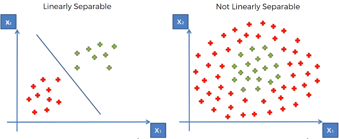
This happens because in this case the data is not linearly set separable.

2.2 Mapping to a Higher Dimension

And now what we want to do is we just want to see that it is indeed linearly separable. And as you can see this dataset became linearly separable in this dimension.

It is possible to do the same thing applies to two-dimensional space moving into three-dimensional space you'd map it into three-dimensional space and then somehow it would become a linearly separable data set in this space and here we've got a new dimension which is Zed and in a three-dimensional space the linear separator is no longer a line. It's a hyperplane.

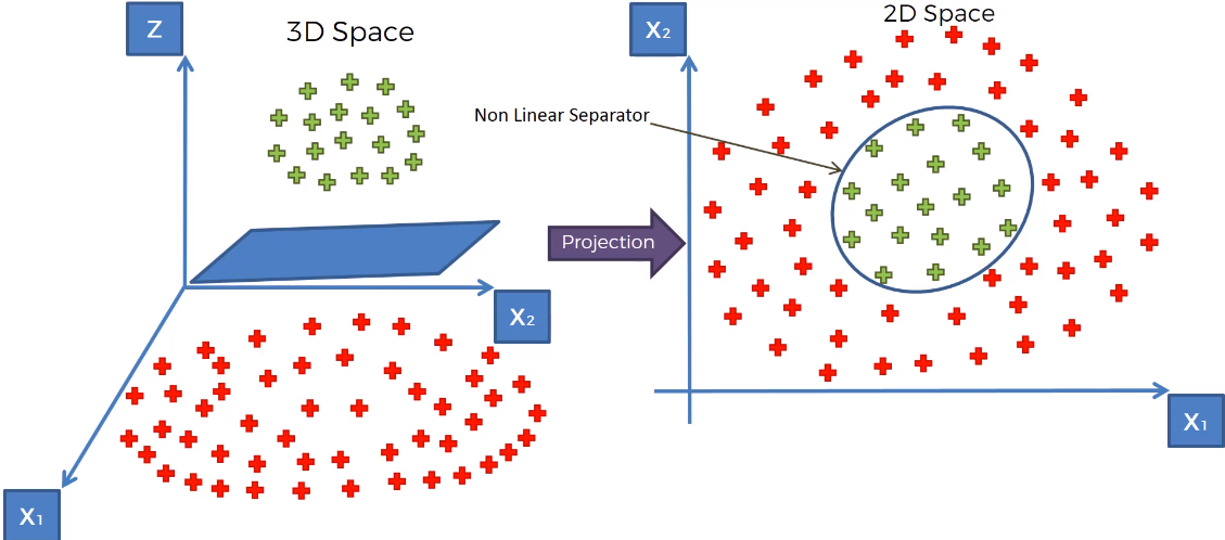
Then we just projected back into our two-dimensional space and we've got this circle that encompasses our classes or surprise or classes and there we go we've got the nonlinear separator.

2.2.1 Drawback

Mapping to a Higher Dimensional Space can be highly computed-intensive. therefore this approach isn't the best because you can imagine like you have a dataset and then mapping it to a higher dimension performing all the calculations there and then coming back to your lower dimension that can even for a computer and on just like in our minds ask as humans but just like for a computer that can cause a lot of delays it can cause a lot of like processing backlog and issues.

2.3 The Kernel Trick

2.3.1 The Gaussian RBF Kernel

$$K(\vec{x},\vec{l}^{i})=e^{-\frac{\left \| \vec{x}-\vec{l}^{i} \right \|^{2}}{2\sigma^{2}}}$$

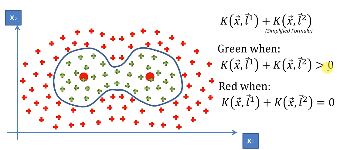
K stands for kernel and it's the function applied to two vectors. The X Factor so this is just some sort of point in our dataset and l stands for Landmark. I mean there might be several landmarks but we're going to we're not going to worry about either.

we've got l, the Landmark is actually in the middle of this plane. So in the middle of this two-dimensional space. And then the vertical here the vertical axis represents the result that we get when we calculate the equation.

So k this distance x - l^i this distance every squaring here will be measured from that landmark. Basically, as you get close to 0 E2 we get closer to E to the power of 0. And each of the power of 0 is 1.

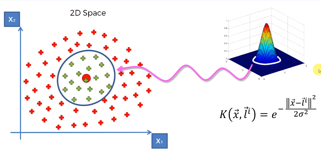
Based on this function it'll get a value of above 0 and that is how we can separate the two classes. The green from the red just if we pick the right Sigma. So here we know that Sigma actually.

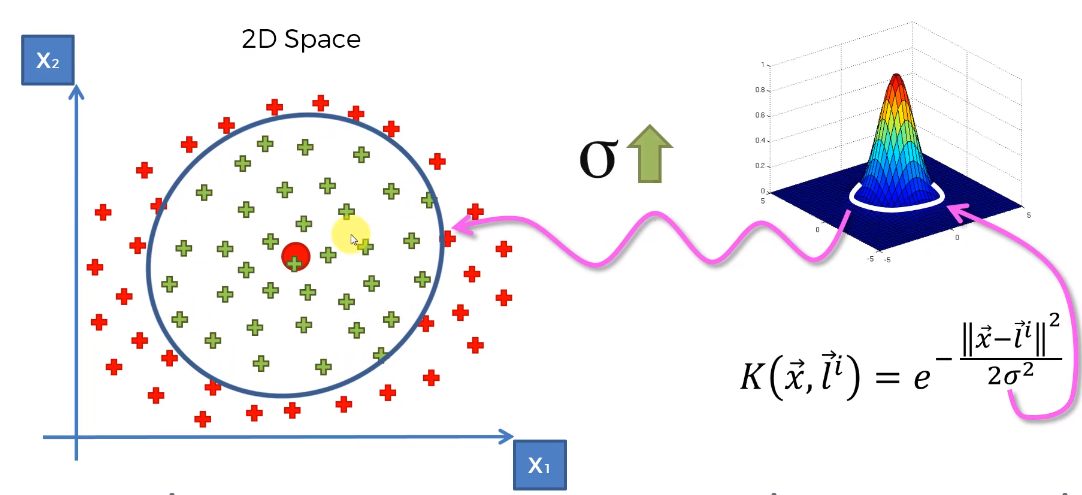
$\sigma$ defines how wide this circumference is. So if you increase sigma the circumference will increase like this picture in shape.

That will allow you to classify each one and that, in essence, is a kernel trick we have created a decision boundary we followed actually going into a higher dimensional space without having to project all of our or create a mapping function that's going to take us two-dimensional space and do all that can be taken. The point is we're not doing that can be stationed in the higher dimensional space we're still doing the computations in the low dimensional space. If we, if you look at the computer, is actually happening and still in the two-dimensional space and that's called the kernel tree.

3. Types of Kernel

4. Example

4.1 Polynomial Kernel

4.2 Radial Kernel

5. Reference

https://thatcher.dev/MLKernels.jl/dev/

https://github.com/trthatcher/MLKernels.jl

https://www.youtube.com/watch?v=efR1C6CvhmE&t=320s

https://www.youtube.com/watch?v=Qc5IyLW_hns